

Step-by-Step Data Integration: Tutorial for Building Robust Star Schema in Data Warehouses
25-08-2024 - Shai Zambrovski
Introduction
In the early days of business data processing, databases were mainly built to manage transactions tied to commercial activities—such as making sales, placing orders, or processing payroll.
These transactions were critical to daily operations, with a focus on ensuring fast and reliable updates to the database as these activities took place.
Over time, the term "transaction" became closely associated with any group of database operations that formed a logical unit of work.
As databases evolved to store a wider variety of data—like user interactions, game activities, or social media comments—the fundamental approach remained transactional.
Applications would typically retrieve and update small amounts of data using specific keys, a method known as online transaction processing (OLTP).
However, as businesses increasingly relied on data for decision-making, a new approach to data access emerged.
This approach focused on analyzing large datasets to extract meaningful insights.
Unlike transactional queries, these analytic queries involved scanning extensive records, performing aggregations, and generating statistics to support business strategy.
This shift led to the development of online analytic processing (OLAP) systems, which were tailored to handle complex queries over large datasets.
By the late 1980s and early 1990s, it became evident that using the same databases for both OLTP and OLAP was not efficient.
To better support the demands of data analysis, organizations began separating their analytic workloads from transactional systems.
This gave rise to the data warehouse—a specialized database designed to store vast amounts of historical data and facilitate robust data analytics and business intelligence.
Five key differences between OLTP and OLAP
| Property | OLTP (Online Transaction Processing) | OLAP (Online Analytical Processing) |
|---|---|---|
| Primary Purpose | Manage day-to-day operations | Support data analysis and decision-making |
| Query Type | Short, simple transactions | Complex queries with aggregations |
| Data Volume | Smaller, often gigabytes to terabytes | Large, often terabytes to petabytes |
| Data Type | Current, real-time data | Historical data, often aggregated |
| User Type | End-users/customers via applications | Analysts and management for insights |
The concept of the data warehouse emerged as businesses began to realize that using the same database for both transactional processing (OLTP) and data analytics (OLAP) was not efficient.
Initially, companies used their OLTP databases for both types of operations—managing day-to-day transactions and running analytic queries.
However, this dual use presented challenges, as OLTP systems are optimized for fast, small transactions, while OLAP requires scanning and aggregating large volumes of data.
As the need for in-depth analysis and decision-making grew, it became clear that separating these workloads would improve performance and efficiency.
This led to the creation of dedicated databases for analytics, known as data warehouses.
These specialized systems were designed to handle large-scale data aggregation and analysis, allowing companies to perform complex queries on historical data without impacting the performance of their transactional systems.
Thus, the data warehouse was born out of the need to support robust data analytics separate from the operational demands of OLTP systems.
Data warehouses were developed as separate databases dedicated to analytical tasks.
These warehouses enable analysts to perform extensive queries without interfering with the OLTP systems.
The data warehouse contains a read-only copy of the data from the organization’s various OLTP systems.
This data is either periodically or continuously extracted from the OLTP systems. It is then either transformed into a structure optimized for analysis before being loaded into the data warehouse (ETL: Extract–Transform–Load) or loaded directly into the warehouse where transformation occurs afterward (ELT: Extract–Load–Transform).
Both methods ensure the data is cleaned and prepared for in-depth analysis.
ETL (Extract–Transform–Load) vs ELT (Extract–Load–Transform)
- ETL (Extract, Transform, Load): A data integration process where data is extracted from sources, transformed into the required format, and then loaded into a target system.
- ELT (Extract, Load, Transform): A data integration process where data is extracted from sources, loaded directly into a target system, and then transformed within the target system.
Differences
| Difference | ETL | ELT |
|---|---|---|
| Order | Transforms before loading | Loads before transforming |
| Processing Location | Uses a staging area | Uses the target system |
| Complexity | Handles complex transformations before loading | Relies on the target system for transformations |
| Performance | May have bottlenecks in the transformation phase | Leverages target system scalability |
| Flexibility | Less flexible for changes | Allows more on-the-fly transformations |
| Cost | May involve additional costs for ETL tools and infrastructure | Typically utilizes existing infrastructure, potentially reducing costs |
| Diagram | 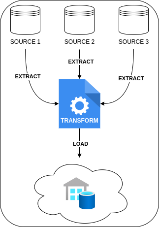 |
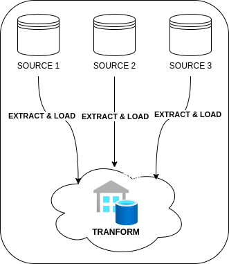 |
Data modeling in data Warehousing: Star Schema
A variety of data models are employed in transaction processing based on application requirements.
Conversely, in analytics, data models are less varied. Many data warehouses utilize a standardized approach called a star schema, or dimensional modeling.
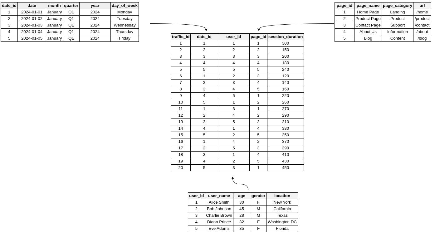
The star schema for web traffic analysis centers around a fact table that captures key events on a website.
In this case, each row in the fact table might represent a significant user action, such as a page view or a click.
This fact table is linked to various dimension tables that provide additional context, such as the date of the event, details about the user, and information about the specific page they interacted with.
These dimensions help in breaking down and analyzing the website's traffic patterns effectively.
In a web traffic star schema, each entry in the fact table represents a specific event, such as a page view or a click, which allows for flexible and detailed analysis.
However, this can result in a very large fact table, especially for high-traffic websites with extensive data.
The fact table includes both attributes—like session duration or click counts—and foreign key references to dimension tables.
These dimension tables provide essential details about the events, answering questions such as who the user was, what page they interacted with, when the event occurred, and more.
For example, one dimension table might include user profiles, while another might describe the pages viewed.
Time is often managed through a dimension table as well, which enables more sophisticated analysis, such as comparing traffic patterns on holidays versus regular days.
The term "star schema" derives from the layout where the fact table is at the center, with dimension tables branching out like the points of a star.
A related design is the snowflake schema, which further breaks down dimension tables into subdimensions for additional normalization.
This could mean having separate tables for brands and product categories, with each referencing these tables rather than storing the details directly.
While snowflake schemas are more normalized, star schemas are favored for their simplicity and ease of use in data analysis.
In a web traffic data warehouse, tables can be very wide,
with fact tables potentially containing hundreds of columns to capture various metrics.
Dimension tables can also be extensive, including detailed metadata such as user demographics, page characteristics, and referral sources, all contributing to comprehensive web traffic analysis.
The Grain of the fact table
Before choosing any dimensions or measurements, the very first design decision of a star schema is declaring the grain - the exact meaning of a single row in the fact table.
In our web traffic example, the grain could be defined in several different ways:
-
One row per page view: The most detailed option, every single page view becomes a row in the fact table.
-
One row per session: A more compact option, each row summarizes an entire visit of a user.
-
One row per page per day: An aggregated option, each row holds the daily totals of a single page.
Each grain answers different business questions - with a daily aggregate we can never analyze the behavior inside a single session, because that detail was thrown away before it reached the warehouse.
That is why the recommended practice is to store the fact table in the finest (atomic) grain that the source systems can provide - we can always aggregate upwards in a query, but we can never drill down below the grain that was stored.
Also, we should never mix different grains in the same fact table - combining page views and daily summaries in one table will lead to double counting and incorrect aggregations.
The Date dimension
The one dimension table that exists in almost every data warehouse is the date dimension - a table with a single row for every calendar day.
Instead of storing just a raw date on each fact row, the fact table references the matching row in the date dimension, which holds pre-computed attributes for that day.
| Date Key | Date | Day of Week | Month | Quarter | Is Weekend | Is Holiday |
|---|---|---|---|---|---|---|
| 20240824 | 2024-08-24 | Saturday | August | Q3 | Yes | No |
| 20240825 | 2024-08-25 | Sunday | August | Q3 | Yes | No |
Each calendar day is a row, enriched with attributes that describe it.
Explanation: Because attributes such as day of week, quarter, weekend and holiday flags are computed once when the dimension is loaded, every analytic query can filter or group by them with a simple join - for example, comparing traffic on holidays versus regular days - without re-calculating date logic in each query. It also guarantees that the entire organization shares the same calendar definitions, such as fiscal periods or which days count as holidays.
The date dimension is also unusually small and predictable - ten years of history are less than four thousand rows - so it is typically generated in advance for both past and future dates.
Why to use Star Schema in data Warehousing?
-
Quicker Aggregations: The straightforward queries of a star schema lead to better performance for aggregation tasks.
-
Easier Query Management: Star schemas offer simpler join logic compared to highly normalized transactional schemas.
-
Streamlined Business Reporting: Star schemas simplify common reporting tasks, such as period-over-period and as-of reporting, compared to more normalized schemas.
-
Enhanced Query Performance: Star schemas can improve performance for read-only reporting applications versus highly normalized schemas.
How to track changes in Star Schema?
In data management and warehousing, a Slowly Changing Dimension (SCD) refers to a type of dimension where the data remains mostly stable but can occasionally change in ways that are hard to predict.
This is different from rapidly changing dimensions, like transactional data (e.g. product price or quantity), which are frequently updated.
Typical examples of SCDs include things like customer address, product description or even employee job title.
Next, I’ll be explaining the six types of Slowly Changing Dimensions (SCD) used in star schema design for data warehouses.
These methods help manage changes to dimensional data over time, from simple updates to more complex ways of keeping history.
SCD Type 0
| Customer ID | Name | Address |
|---|---|---|
| 1 | John Doe | 123 Elm St |
No changes tracked; the initial data remains unchanged.
Explanation: SCD Type 0 does not track any changes to the data. The dimension is static, and once the data is loaded into the system, it remains as is. This approach is suitable for data that does not change or where historical changes are not important.
SCD Type 1
| Customer ID | Name | Address |
|---|---|---|
| 1 | John Doe | 456 Oak St |
Old data is overwritten with the new data.
Explanation: SCD Type 1 involves overwriting the existing data with new data. This approach does not preserve any history of changes; the most recent data is all that is retained. It is best used when only the current state of the data is relevant, and historical changes are not needed.
SCD Type 2
| Customer ID | Name | Address | Effective Date | Expiry Date |
|---|---|---|---|---|
| 1 | John Doe | 123 Elm St | 2022-01-01 | 2024-01-01 |
| 1 | John Doe | 456 Oak St | 2024-01-02 | NULL |
Tracks historical changes by adding new rows for each change.
Explanation: SCD Type 2 tracks historical changes by creating a new row for each change. It includes additional columns to capture the dates when the data was valid (Effective Date and Expiry Date). This approach is useful for maintaining a full history of changes and is commonly used when it's important to analyze historical data.
SCD Type 3
| Customer ID | Name | Current Address | Previous Address |
|---|---|---|---|
| 1 | John Doe | 456 Oak St | 123 Elm St |
Stores current and one previous version of the data.
Explanation: SCD Type 3 keeps track of the current data and one previous version by adding extra columns for the old values. This method allows for some historical tracking but is limited to only the most recent past. It's suitable for scenarios where only the immediate past changes are relevant.
SCD Type 4
Main Dimension Table:
| Customer ID | Name | Address |
|---|---|---|
| 1 | John Doe | 456 Oak St |
Historical Data Table:
| Customer ID | Address | Change Date |
|---|---|---|
| 1 | 123 Elm St | 2022-01-01 |
| 1 | 456 Oak St | 2024-01-02 |
Stores historical data in a separate table.
Explanation: SCD Type 4 separates current data from historical data by maintaining two tables. The main dimension table holds the current data, while a separate historical table records changes over time. This approach is beneficial for managing large datasets where maintaining history separately can optimize performance.
SCD Type 5
Main Dimension Table:
| Customer ID | Name | Current Address | Previous Address | Address Change Flag |
|---|---|---|---|---|
| 1 | John Doe | 456 Oak St | 123 Elm St | Yes |
Historical Data Table:
| Customer ID | Address | Change Date |
|---|---|---|
| 1 | 123 Elm St | 2022-01-01 |
| 1 | 456 Oak St | 2024-01-02 |
Explanation: SCD Type 5 combines elements of SCD Types 1 and 2. It keeps the current data in the main dimension table and maintains a historical record in a separate table. Additionally, it includes a flag or indicator (e.g., Address Change Flag) to signify whether a change has occurred. This approach provides a balance between maintaining a history of changes and managing current data efficiently, especially when changes are infrequent but important to track.
SCD Type 6
Main Dimension Table:
| Customer ID | Name | Current Address | Previous Address |
|---|---|---|---|
| 1 | John Doe | 456 Oak St | 123 Elm St |
Historical Data Table:
| Customer ID | Address | Change Date |
|---|---|---|
| 1 | 123 Elm St | 2022-01-01 |
| 1 | 456 Oak St | 2024-01-02 |
Combines aspects of Types 1, 2, and 3 by preserving current and historical data through both new rows and new columns.
Explanation: SCD Type 6 integrates elements of Types 1, 2, and 3. It maintains current data in the main dimension table while preserving historical changes in a separate table and through additional columns. This hybrid approach offers flexibility, allowing for detailed historical analysis while keeping the most relevant current data readily accessible.
It's all about Surrogate keys
After reviewing the SCD types, one question remains - if the same customer can appear in the dimension table multiple times (as we saw in SCD Type 2), how can the fact table reference the correct version of that customer?
The answer is the surrogate key.
A surrogate key is an artificial key - usually a simple sequential number - that is generated by the data warehouse itself and has no business meaning at all.
It stands in contrast to the natural key (also called a business key), which is the identifier that comes from the source OLTP system, such as the Customer ID in our examples.
| Customer Key (Surrogate) | Customer ID (Natural) | Name | Address | Effective Date | Expiry Date |
|---|---|---|---|---|---|
| 1001 | 1 | John Doe | 123 Elm St | 2022-01-01 | 2024-01-01 |
| 1002 | 1 | John Doe | 456 Oak St | 2024-01-02 | NULL |
The fact table references the surrogate key (Customer Key), not the natural key (Customer ID).
Explanation: Both rows describe the same customer (natural key 1), but each version of the customer gets its own surrogate key. A fact row that was loaded while John Doe lived at 123 Elm St will point to surrogate key 1001, while newer fact rows will point to 1002. This way, every fact is permanently connected to the version of the dimension that was true when the event happened.
There are several reasons why we will always prefer surrogate keys over natural keys in a star schema:
-
History tracking: As we saw, SCD Type 2 creates multiple rows for the same business entity. The natural key is no longer unique in the dimension table, so it simply cannot be used as the primary key.
-
Decoupling from the source systems: The data warehouse does not control the OLTP systems. Natural keys can be changed, recycled or reused by the source application, and such a change would silently corrupt the warehouse. A surrogate key is owned by the warehouse and will never change.
-
Integrating multiple sources: When the warehouse loads data from several OLTP systems, two different systems can easily use the same natural key for two different entities (for example, customer 1 in the CRM and customer 1 in the billing system). Surrogate keys eliminate those collisions.
-
Performance: Surrogate keys are small integers, which makes the joins between the huge fact table and the dimension tables faster and the fact table itself narrower, compared to joining on long strings or composite natural keys.
-
Handling unknown or missing data: We can reserve special surrogate key values for cases like "unknown customer" or "not applicable", so fact rows never need to hold NULL foreign keys.
The natural key is still stored in the dimension table as a regular attribute - it is essential for the ETL/ELT process to match incoming source records to the correct dimension rows, and for tracing a dimension row back to its origin system.